Spectral density

In statistical signal processing and physics, the spectral density, power spectral density (PSD), or energy spectral density (ESD), is a positive real function of a frequency variable associated with a stationary stochastic process, or a deterministic function of time, which has dimensions of power per hertz (Hz), or energy per hertz. It is often called simply the spectrum of the signal. Intuitively, the spectral density measures the frequency content of a stochastic process and helps identify periodicities.

1 Explanation
2 Definition
3 Estimation
4 Properties
5 Related concepts
6 Applications
- 6.1 Electrical engineering
- 6.2 Coherence
7 See also
8 References

Explanation

In physics, the signal is usually a wave, such as an electromagnetic wave, random vibration, or an acoustic wave. The spectral density of the wave, when multiplied by an appropriate factor, will give the power carried by the wave, per unit frequency, known as the power spectral density (PSD) of the signal. Power spectral density is commonly expressed in watts per hertz (W/Hz)^[1] or dBm/Hz.

For voltage signals, it is customary to use units of V²Hz⁻¹ for PSD, and V²sHz⁻¹ for ESD^[2] or dBμV/Hz.

For random vibration analysis, units of g²Hz⁻¹ are sometimes used for acceleration spectral density.^[3]

Although it is not necessary to assign physical dimensions to the signal or its argument, in the following discussion the terms used will assume that the signal varies in time.

Definition

Energy spectral density

The energy spectral density describes how the energy (or variance) of a signal or a time series is distributed with frequency. If $f(t)$ is a finite-energy (square integrable) signal, the spectral density $\Phi(\omega)$ of the signal is the square of the magnitude of the continuous Fourier transform of the signal (here energy is taken as the integral of the square of a signal, which is the same as physical energy if the signal is a voltage applied to a 1-ohm load, or the current).

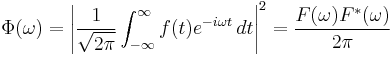
$\Phi(\omega)=\left|\frac{1}{\sqrt{2\pi}}\int_{-\infty}^\infty f(t)e^{-i\omega t}\,dt\right|^2 = \frac{F(\omega)F^*(\omega)}{2\pi}$

where $\omega$ is the angular frequency ( $2\pi$ times the ordinary frequency) and $F(\omega)$ is the continuous Fourier transform of $f(t)$ , and $F^*(\omega)$ is its complex conjugate.

If the signal is discrete with values $f_n$ , over an infinite number of elements, we still have an energy spectral density:

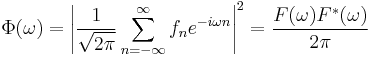
$\Phi(\omega)=\left|\frac{1}{\sqrt{2\pi}}\sum_{n=-\infty}^\infty f_n e^{-i\omega n}\right|^2=\frac{F(\omega)F^*(\omega)}{2\pi}$

where $F(\omega)$ is the discrete-time Fourier transform of $f_n$ .

If the number of defined values is finite, the sequence does not have an energy spectral density per se, but the sequence can be treated as periodic, using a Discrete Fourier Transform (DFT) to make a discrete spectrum, or it can be extended with zeros and a spectral density can be computed as in the infinite-sequence case.

The continuous and discrete spectral densities are often denoted with the same symbols, as above, though their dimensions and units differ; the continuous case has a time-squared factor that the discrete case does not have. They can be made to have equal dimensions and units by measuring time in units of sample intervals or by scaling the discrete case to the desired time units.

As is always the case, the multiplicative factor of $1/2\pi$ is not absolute, but rather depends on the particular normalizing constants used in the definition of the various Fourier transforms.

Power spectral density

The above definitions of energy spectral density require that the Fourier transforms of the signals exist, that is, that the signals are integrable/summable or square-integrable/square-summable. (Note: The integral definition of the Fourier transform is only well-defined when the function is integrable. It is not sufficient for a function to be simply square-integrable. In this case one would need to use the Plancherel theorem.) An often more useful alternative is the power spectral density (PSD), which describes how the power of a signal or time series is distributed with frequency. Here power can be the actual physical power, or more often, for convenience with abstract signals, can be defined as the squared value of the signal, that is, as the actual power dissipated in a purely resistive load if the signal were a voltage applied across it. This instantaneous power (the mean or expected value of which is the average power) is then given by

$P(t) = s(t)^2$

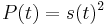
for a signal $s(t)$ .

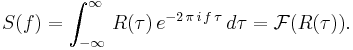
Since a signal with nonzero average power is not square integrable, the Fourier transforms do not exist in this case. Fortunately, the Wiener–Khinchin theorem provides a simple alternative. The PSD is the Fourier transform of the autocorrelation function, $R(\tau)$ , of the signal if the signal is treated as a wide-sense stationary random process.^[4]

These results are expressed in the mathematical formula,

$S(f)=\int_{-\infty}^\infty \,R(\tau)\,e^{-2\,\pi\,i\,f\,\tau}\,d \tau=\mathcal{F}(R(\tau)).$

The ensemble average of the average periodogram when the averaging time interval T→∞ can be proved (Brown & Hwang^[5]) to approach the Power Spectral Density (PSD):

$E\left[\frac{|\mathcal{F}(f_T(t))|^2}{T}\right] \to S(f)$

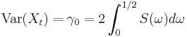
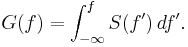
The power of the signal in a given frequency band can be calculated by integrating over positive and negative frequencies,

$P=\int_{F_1}^{F_2}\,S(f)\,d f %2B \int_{-F_2}^{-F_1}\,S(f)\,df.$

The power spectral density of a signal exists if the signal is a wide-sense stationary process. If the signal is not wide-sense stationary, then the autocorrelation function must be a function of two variables. In some cases, such as wide-sense cyclostationary processes, a PSD may still exist.^[6] More generally, similar techniques may be used to estimate a time-varying spectral density.

If two signals both possess power spectra (the correct terminology), then a cross-power spectrum can be calculated by using their cross-correlation function.

Properties of the power spectral density

^[7]spectrum of a real valued process is symmetric: $S(-f) = S(f)$
is continuous and differentiable on [-1/2, +1/2]
derivative is zero at f = 0
auto-covariance can be reconstructed by using the Inverse Fourier transform
describes the distribution of variance across time scales. In particular

$\text{Var}(X_t) = \gamma_0 = 2 \int_0^{1/2} S(\omega) d\omega$
is a linear function of the auto-covariance function

If $\gamma$ is decomposed into two functions $\gamma(\tau) = \alpha_1 \gamma_1(\tau) %2B \alpha_1 \gamma_2(\tau)$ then

$S(f) = \alpha_1 S_1(f) %2B \alpha_2 S_2(f)$

where $S_i(f) = \mathcal{F}\{ \gamma_i \}$

The power spectrum $G(f)$ is defined as^[8]

$G(f)= \int _{-\infty}^f S(f^\prime) \, df^\prime.$

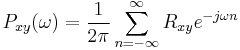
Cross-spectral density

"Just as the Power Spectral Density (PSD) is the Fourier transform of the auto-covariance function we may define the Cross Spectral Density (CSD) as the Fourier transform of the cross-covariance function."^[9]
The PSD is a special case of the cross spectral density (CPSD) function, defined between two signals xⁿ and yⁿ as

$P_{xy}(\omega)=\frac{1}{2\pi}\sum_{n=-\infty}^\infty R_{xy}e^{-j\omega n}$

Estimation

Main article: Spectral density estimation

The goal of spectral density estimation is to estimate the spectral density of a random signal from a sequence of time samples. Depending on what is known about the signal, estimation techniques can involve parametric or non-parametric approaches, and may be based on time-domain or frequency-domain analysis. For example, a common parametric technique involves fitting the observations to an autoregressive model. A common non-parametric technique is the periodogram.

The spectral density is usually estimated using Fourier transform methods, but other techniques such as Welch's method and the maximum entropy method can also be used.

Properties

The spectral density of $f(t)$ and the autocorrelation of $f(t)$ form a Fourier transform pair (for PSD versus ESD, different definitions of autocorrelation function are used).

One of the results of Fourier analysis is Parseval's theorem which states that the area under the energy spectral density curve is equal to the area under the square of the magnitude of the signal, the total energy:

$\int_{-\infty}^\infty \left| f(t) \right|^2\, dt = \int_{-\infty}^\infty \Phi(\omega)\, d\omega.$

The above theorem holds true in the discrete cases as well. A similar result holds for the total power in a power spectral density being equal to the corresponding mean total signal power, which is the autocorrelation function at zero lag.

Related concepts

Most "frequency" graphs really display only the spectral density. Sometimes the complete frequency spectrum is graphed in 2 parts, "amplitude" versus frequency (which is the spectral density) and "phase" versus frequency (which contains the rest of the information from the frequency spectrum). $f(t)$ cannot be recovered from the spectral density part alone — the "temporal information" is lost.

The spectral centroid of a signal is the midpoint of its spectral density function, i.e. the frequency that divides the distribution into two equal parts.

The spectral edge frequency of a signal is an extension of the previous concept to any proportion instead of two equal parts.

Spectral density is a function of frequency, not a function of time. However, the spectral density of small "windows" of a longer signal may be calculated, and plotted versus time associated with the window. Such a graph is called a spectrogram. This is the basis of a number of spectral analysis techniques such as the short-time Fourier transform and wavelets.

In radiometry and colorimetry (or color science more generally), the spectral power distribution (SPD) of a light source is a measure of the power carried by each frequency or "color" in a light source. The light spectrum is usually measured at points (often 31) along the visible spectrum, in wavelength space instead of frequency space, which makes it not strictly a spectral density. Some spectrophotometers can measure increments as fine as 1 or 2 nanometers. Values are used to calculate other specifications and then plotted to demonstrate the spectral attributes of the source. This can be a helpful tool in analyzing the color characteristics of a particular source.

Applications

Electrical engineering

The concept and use of the power spectrum of a signal is fundamental in electrical engineering, especially in electronic communication systems, including radio communications, radars, and related systems, plus passive [remote sensing] technology. Much effort has been expended and millions of dollars spent on developing and producing electronic instruments called "spectrum analyzers" for aiding electrical engineers and technicians in observing and measuring the power spectra of signals. The cost of a spectrum analyzer varies depending on its frequency range, its bandwidth (signal processing), and its accuracy. The higher the frequency range (S-band, C-band, X-band, Ku-band, K-band, Ka-band, etc.), the more difficult the components are to make, and the more expensive the spectrum analyzer is. Also, the wider the bandwidth that a spectrum analyzer possesses, the more costly that it is, and the capability for more accurate measurements increases costs as well.

The spectrum analyzer measures the magnitude of the short-time Fourier transform (STFT) of an input signal. If the signal being analyzed can be considered a stationary process, the STFT is a good smoothed estimate of its power spectral density.

Coherence

See Coherence (signal processing) for use of the cross-spectral density.

References

^ Gérard Maral (2003). VSAT Networks. John Wiley and Sons. ISBN 0470866845. http://books.google.com/books?id=CMx5HQ1Mr_UC&pg=PR20&dq=%22power+spectral+density%22+W/Hz&lr=&as_brr=0&ei=VYwvSImyA4L4sQPxxJXzAg&sig=-bko0DhmJwzISN6PcHszF9E3qUE#PPR20,M1.
^ Michael Peter Norton and Denis G. Karczub (2003). Fundamentals of Noise and Vibration Analysis for Engineers. Cambridge University Press. ISBN 0521499135. http://books.google.com/books?id=jDeRCSqtev4C&pg=PA352&dq=%22power+spectral+density%22+%22energy+spectral+density%22&lr=&as_brr=3&ei=i3IvSLL6H4-KsgPfze13&sig=RJgA8uGocYf5d6mC6rKKS-X_2bc.
^ Alessandro Birolini (2007). Reliability Engineering. Springer. p. 83. ISBN 9783540493884. http://books.google.com/books?id=xPIW3AI9tdAC&pg=PA83&dq=acceleration-spectral-density+g+hz&as_brr=3&ei=q24xSpKOBZXkzASPrs39BQ.
^ Dennis Ward Ricker (2003). Echo Signal Processing. Springer. ISBN 140207395X. http://books.google.com/books?id=NF2Tmty9nugC&pg=PA23&dq=%22power+spectral+density%22+%22energy+spectral+density%22&lr=&as_brr=3&ei=HZMvSPSWFZyStwPWsfyBAw&sig=1ZZcHwxXkErvNXtAHv21ijTXoP8#PPA23,M1.
^ Robert Grover Brown & Patrick Y.C. Hwang (1997). Introduction to Random Signals and Applied Kalman Filtering. John Wiley & Sons. ISBN 0471128392. http://www.amazon.com/dp/0471128392.
^ Andreas F. Molisch (2011). Wireless Communications (2nd ed.). John Wiley and Sons. p. 194. ISBN 9780470741870. http://books.google.com/books?id=vASyH5-jfMYC&pg=PA194.
^ Storch, H. Von; F. W Zwiers (2001). Statistical analysis in climate research. Cambridge Univ Pr. ISBN 0521012309.
^ An Introduction to the Theory of Random Signals and Noise, Wilbur B. Davenport and Willian L. Root, IEEE Press, New York, 1987, ISBN 0-87942-235-1
^ http://www.fil.ion.ucl.ac.uk/~wpenny/course/course.html, chapter 7